The term cluster validation is used to design the procedure of evaluating the goodness of clustering algorithm results. This is important to avoid finding patterns in a random data, as well as, in the situation where you want to compare two clustering algorithms.
Generally, clustering validation statistics can be categorized into 3 classes (Charrad et al. 2014,Brock et al. (2008), Theodoridis and Koutroumbas (2008)):
- Internal cluster validation, which uses the internal information of the clustering process to evaluate the goodness of a clustering structure without reference to external information. It can be also used for estimating the number of clusters and the appropriate clustering algorithm without any external data.
- External cluster validation, which consists in comparing the results of a cluster analysis to an externally known result, such as externally provided class labels. It measures the extent to which cluster labels match externally supplied class labels. Since we know the “true” cluster number in advance, this approach is mainly used for selecting the right clustering algorithm for a specific data set.
- Relative cluster validation, which evaluates the clustering structure by varying different parameter values for the same algorithm (e.g.,: varying the number of clusters k). It’s generally used for determining the optimal number of clusters.
In this chapter, we start by describing the different methods for clustering validation. Next, we’ll demonstrate how to compare the quality of clustering results obtained with different clustering algorithms. Finally, we’ll provide R scripts for validating clustering results.
In all the examples presented here, we’ll apply k-means, PAM and hierarchical clustering. Note that, the functions used in this article can be applied to evaluate the validity of any other clustering methods.
Contents:
Related Book
Practical Guide to Cluster Analysis in RInternal measures for cluster validation
In this section, we describe the most widely used clustering validation indices. Recall that the goal of partitioning clustering algorithms (Part @ref(partitioning-clustering)) is to split the data set into clusters of objects, such that:
- the objects in the same cluster are similar as much as possible,
- and the objects in different clusters are highly distinct
That is, we want the average distance within cluster to be as small as possible; and the average distance between clusters to be as large as possible.
Internal validation measures reflect often the compactness, the connectedness and the separation of the cluster partitions.
- Compactness or cluster cohesion: Measures how close are the objects within the same cluster. A lower within-cluster variation is an indicator of a good compactness (i.e., a good clustering). The different indices for evaluating the compactness of clusters are base on distance measures such as the cluster-wise within average/median distances between observations.
- Separation: Measures how well-separated a cluster is from other clusters. The indices used as separation measures include:
- distances between cluster centers
- the pairwise minimum distances between objects in different clusters
- Connectivity: corresponds to what extent items are placed in the same cluster as their nearest neighbors in the data space. The connectivity has a value between 0 and infinity and should be minimized.
Generally most of the indices used for internal clustering validation combine compactness and separation measures as follow:
\[
Index = \frac{(\alpha \times Separation)}{(\beta \times Compactness)}
\]
Where \(\alpha\) and \(\beta\) are weights.
In this section, we’ll describe the two commonly used indices for assessing the goodness of clustering: the silhouette width and the Dunn index. These internal measure can be used also to determine the optimal number of clusters in the data.
Silhouette coefficient
The silhouette analysis measures how well an observation is clustered and it estimates the average distance between clusters. The silhouette plot displays a measure of how close each point in one cluster is to points in the neighboring clusters.
For each observation \(i\), the silhouette width \(s_i\) is calculated as follows:
- For each observation \(i\), calculate the average dissimilarity \(a_i\) between \(i\) and all other points of the cluster to which i belongs.
- For all other clusters \(C\), to which i does not belong, calculate the average dissimilarity \(d(i, C)\) of \(i\) to all observations of C. The smallest of these \(d(i,C)\) is defined as \(b_i= \min_C d(i,C)\). The value of \(b_i\) can be seen as the dissimilarity between \(i\) and its “neighbor” cluster, i.e., the nearest one to which it does not belong.
- Finally the silhouette width of the observation \(i\) is defined by the formula: \(S_i = (b_i - a_i)/max(a_i, b_i)\).
Silhouette width can be interpreted as follow:
- Observations with a large Si (almost 1) are very well clustered.
- A small Si (around 0) means that the observation lies between two clusters.
- Observations with a negative Si are probably placed in the wrong cluster.
Dunn index
The Dunn index is another internal clustering validation measure which can be computed as follow:
- For each cluster, compute the distance between each of the objects in the cluster and the objects in the other clusters
- Use the minimum of this pairwise distance as the inter-cluster separation (min.separation)
- For each cluster, compute the distance between the objects in the same cluster.
- Use the maximal intra-cluster distance (i.e maximum diameter) as the intra-cluster compactness
- Calculate the Dunn index (D) as follow:
\[
D = \frac{min.separation}{max.diameter}
\]
If the data set contains compact and well-separated clusters, the diameter of the clusters is expected to be small and the distance between the clusters is expected to be large. Thus, Dunn index should be maximized.
External measures for clustering validation
The aim is to compare the identified clusters (by k-means, pam or hierarchical clustering) to an external reference.
It’s possible to quantify the agreement between partitioning clusters and external reference using either the corrected Rand index and Meila’s variation index VI, which are implemented in the R function cluster.stats()[fpc package].
The corrected Rand index varies from -1 (no agreement) to 1 (perfect agreement).
External clustering validation, can be used to select suitable clustering algorithm for a given data set.
Computing cluster validation statistics in R
Required R packages
The following R packages are required in this chapter:
- factoextra for data visualization
- fpc for computing clustering validation statistics
- NbClust for determining the optimal number of clusters in the data set.
- Install the packages:
install.packages(c("factoextra", "fpc", "NbClust"))- Load the packages:
library(factoextra)
library(fpc)
library(NbClust)
Data preparation
We’ll use the built-in R data set iris:
# Excluding the column "Species" at position 5
df <- iris[, -5]
# Standardize
df <- scale(df)
Clustering analysis
We’ll use the function eclust() [enhanced clustering, in factoextra] which provides several advantages:
- It simplifies the workflow of clustering analysis
- It can be used to compute hierarchical clustering and partitioning clustering in a single line function call
- Compared to the standard partitioning functions (kmeans, pam, clara and fanny) which requires the user to specify the optimal number of clusters, the function eclust() computes automatically the gap statistic for estimating the right number of clusters.
- It provides silhouette information for all partitioning methods and hierarchical clustering
- It draws beautiful graphs using ggplot2
The simplified format the eclust() function is as follow:
eclust(x, FUNcluster = "kmeans", hc_metric = "euclidean", ...)- x: numeric vector, data matrix or data frame
- FUNcluster: a clustering function including “kmeans”, “pam”, “clara”, “fanny”, “hclust”, “agnes” and “diana”. Abbreviation is allowed.
- hc_metric: character string specifying the metric to be used for calculating dissimilarities between observations. Allowed values are those accepted by the function dist() [including “euclidean”, “manhattan”, “maximum”, “canberra”, “binary”, “minkowski”] and correlation based distance measures [“pearson”, “spearman” or “kendall”]. Used only when FUNcluster is a hierarchical clustering function such as one of “hclust”, “agnes” or “diana”.
- …: other arguments to be passed to FUNcluster.
The function eclust() returns an object of class eclust containing the result of the standard function used (e.g., kmeans, pam, hclust, agnes, diana, etc.).
It includes also:
- cluster: the cluster assignment of observations after cutting the tree
- nbclust: the number of clusters
- silinfo: the silhouette information of observations
- size: the size of clusters
- data: a matrix containing the original or the standardized data (if stand = TRUE)
- gap_stat: containing gap statistics
To compute a partitioning clustering, such as k-means clustering with k = 3, type this:
# K-means clustering
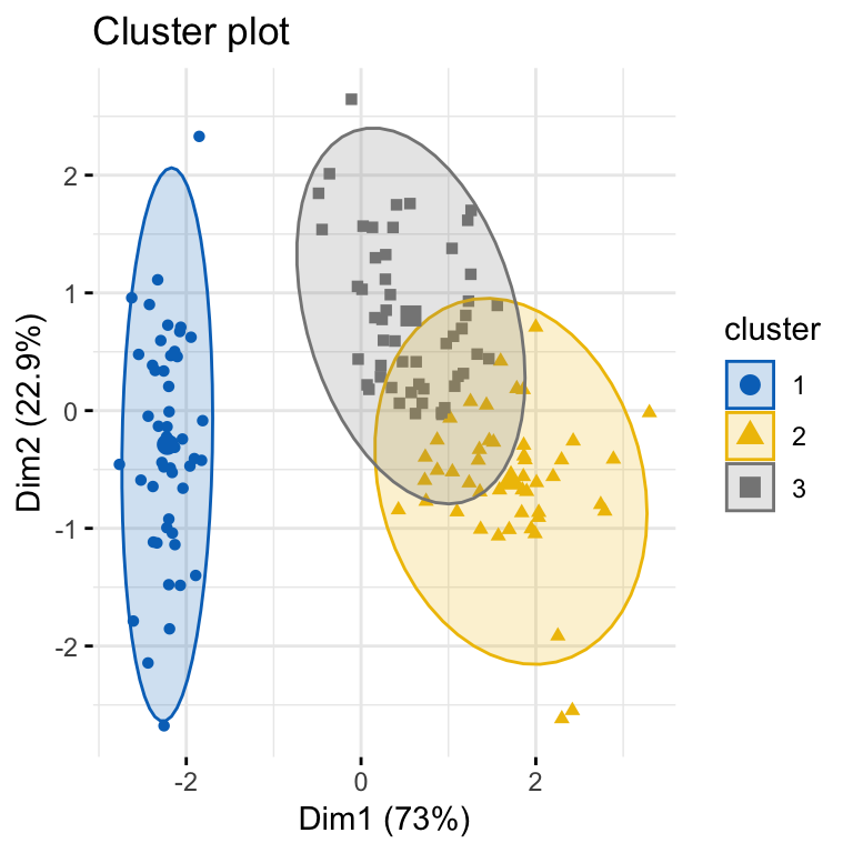
km.res <- eclust(df, "kmeans", k = 3, nstart = 25, graph = FALSE)
# Visualize k-means clusters
fviz_cluster(km.res, geom = "point", ellipse.type = "norm",
             palette = "jco", ggtheme = theme_minimal())
To compute a hierarchical clustering, use this:
# Hierarchical clustering
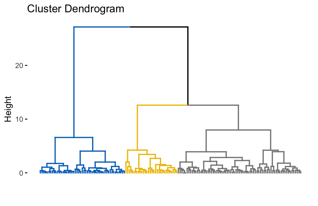
hc.res <- eclust(df, "hclust", k = 3, hc_metric = "euclidean",
                 hc_method = "ward.D2", graph = FALSE)

# Visualize dendrograms
fviz_dend(hc.res, show_labels = FALSE,
         palette = "jco", as.ggplot = TRUE)
Clustering validation
Silhouette plot
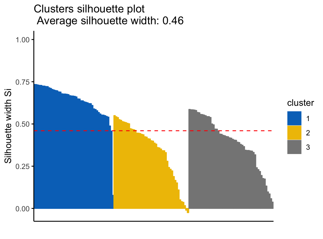
Recall that the silhouette coefficient (\(S_i\)) measures how similar an object \(i\) is to the the other objects in its own cluster versus those in the neighbor cluster. \(S_i\) values range from 1 to - 1:
- A value of \(S_i\) close to 1 indicates that the object is well clustered. In the other words, the object \(i\) is similar to the other objects in its group.
- A value of \(S_i\) close to -1 indicates that the object is poorly clustered, and that assignment to some other cluster would probably improve the overall results.
It’s possible to draw silhouette coefficients of observations using the function fviz_silhouette() [factoextra package], which will also print a summary of the silhouette analysis output. To avoid this, you can use the option print.summary = FALSE.
Claim Your Membership Now
##   cluster size ave.sil.width
## 1       1   50          0.64
## 2       2   47          0.35
## 3       3   53          0.39
Silhouette information can be extracted as follow:
# Silhouette information
silinfo <- km.res$silinfo
names(silinfo)
# Silhouette widths of each observation
head(silinfo$widths[, 1:3], 10)
# Average silhouette width of each cluster
silinfo$clus.avg.widths
# The total average (mean of all individual silhouette widths)
silinfo$avg.width
# The size of each clusters
km.res$size
It can be seen that several samples, in cluster 2, have a negative silhouette coefficient. This means that they are not in the right cluster. We can find the name of these samples and determine the clusters they are closer (neighbor cluster), as follow:
# Silhouette width of observation
sil <- km.res$silinfo$widths[, 1:3]
# Objects with negative silhouette
neg_sil_index <- which(sil[, 'sil_width'] < 0)
sil[neg_sil_index, , drop = FALSE]
## cluster neighbor sil_width
## 112 2 3 -0.0106
## 128 2 3 -0.0249Validation statistics
The function cluster.stats() [fpc package] and the function NbClust() [in NbClust package] can be used to compute Dunn index and many other cluster validation statistics or indices.
The simplified format is:
cluster.stats(d = NULL, clustering, al.clustering = NULL)- d: a distance object between cases as generated by the dist() function
- clustering: vector containing the cluster number of each observation
- alt.clustering: vector such as for clustering, indicating an alternative clustering
The function cluster.stats() returns a list containing many components useful for analyzing the intrinsic characteristics of a clustering:
- cluster.number: number of clusters
- cluster.size: vector containing the number of points in each cluster
- average.distance, median.distance: vector containing the cluster-wise within average/median distances
- average.between: average distance between clusters. We want it to be as large as possible
- average.within: average distance within clusters. We want it to be as small as possible
- clus.avg.silwidths: vector of cluster average silhouette widths. Recall that, the silhouette width is also an estimate of the average distance between clusters. Its value is comprised between 1 and -1 with a value of 1 indicating a very good cluster.
- within.cluster.ss: a generalization of the within clusters sum of squares (k-means objective function), which is obtained if d is a Euclidean distance matrix.
- dunn, dunn2: Dunn index
- corrected.rand, vi: Two indexes to assess the similarity of two clustering: the corrected Rand index and Meila’s VI
All the above elements can be used to evaluate the internal quality of clustering.
In the following sections, we’ll compute the clustering quality statistics for k-means. Look at the within.cluster.ss (within clusters sum of squares), the average.within (average distance within clusters) and clus.avg.silwidths (vector of cluster average silhouette widths).
library(fpc)
# Statistics for k-means clustering
km_stats <- cluster.stats(dist(df),  km.res$cluster)
# Dun index
km_stats$dunn
## [1] 0.0265To display all statistics, type this:
km_statsRead the documentation of cluster.stats() for details about all the available indices.
External clustering validation
Among the values returned by the function cluster.stats(), there are two indexes to assess the similarity of two clustering, namely the corrected Rand index and Meila’s VI.
We know that the iris data contains exactly 3 groups of species.
Does the K-means clustering matches with the true structure of the data?
We can use the function cluster.stats() to answer to this question.
Let start by computing a cross-tabulation between k-means clusters and the reference Species labels:
table(iris$Species, km.res$cluster)##
## 1 2 3
## setosa 50 0 0
## versicolor 0 11 39
## virginica 0 36 14It can be seen that:
- All setosa species (n = 50) has been classified in cluster 1
- A large number of versicor species (n = 39 ) has been classified in cluster 3. Some of them ( n = 11) have been classified in cluster 2.
- A large number of virginica species (n = 36 ) has been classified in cluster 2. Some of them (n = 14) have been classified in cluster 3.
It’s possible to quantify the agreement between Species and k-means clusters using either the corrected Rand index and Meila’s VI provided as follow:
library("fpc")
# Compute cluster stats
species <- as.numeric(iris$Species)
clust_stats <- cluster.stats(d = dist(df),
                             species, km.res$cluster)
# Corrected Rand index
clust_stats$corrected.rand
## [1] 0.62# VI
clust_stats$vi## [1] 0.748The corrected Rand index provides a measure for assessing the similarity between two partitions, adjusted for chance. Its range is -1 (no agreement) to 1 (perfect agreement). Agreement between the specie types and the cluster solution is 0.62 using Rand index and 0.748 using Meila’s VI.
The same analysis can be computed for both PAM and hierarchical clustering:
# Agreement between species and pam clusters
pam.res <- eclust(df, "pam", k = 3, graph = FALSE)
table(iris$Species, pam.res$cluster)
cluster.stats(d = dist(iris.scaled),
              species, pam.res$cluster)$vi
# Agreement between species and HC clusters
res.hc <- eclust(df, "hclust", k = 3, graph = FALSE)
table(iris$Species, res.hc$cluster)
cluster.stats(d = dist(iris.scaled),
              species, res.hc$cluster)$vi
External clustering validation, can be used to select suitable clustering algorithm for a given data set.
Summary
We described how to validate clustering results using the silhouette method and the Dunn index. This task is facilitated using the combination of two R functions: eclust() and fviz_silhouette in the factoextra package We also demonstrated how to assess the agreement between a clustering result and an external reference.
In the next chapters, we’ll show how to i) choose the appropriate clustering algorithm for your data; and ii) computing p-values for hierarchical clustering.
References
Brock, Guy, Vasyl Pihur, Susmita Datta, and Somnath Datta. 2008. “ClValid: An R Package for Cluster Validation.” Journal of Statistical Software 25 (4): 1–22. https://www.jstatsoft.org/v025/i04.
Charrad, Malika, Nadia Ghazzali, Véronique Boiteau, and Azam Niknafs. 2014. “NbClust: An R Package for Determining the Relevant Number of Clusters in a Data Set.” Journal of Statistical Software 61: 1–36. http://www.jstatsoft.org/v61/i06/paper.
Theodoridis, Sergios, and Konstantinos Koutroumbas. 2008. Pattern Recognition. 2nd ed. Academic Press.
Recommended for you
This section contains best data science and self-development resources to help you on your path.
Books - Data Science
Our Books
- Practical Guide to Cluster Analysis in R by A. Kassambara (Datanovia)
- Practical Guide To Principal Component Methods in R by A. Kassambara (Datanovia)
- Machine Learning Essentials: Practical Guide in R by A. Kassambara (Datanovia)
- R Graphics Essentials for Great Data Visualization by A. Kassambara (Datanovia)
- GGPlot2 Essentials for Great Data Visualization in R by A. Kassambara (Datanovia)
- Network Analysis and Visualization in R by A. Kassambara (Datanovia)
- Practical Statistics in R for Comparing Groups: Numerical Variables by A. Kassambara (Datanovia)
- Inter-Rater Reliability Essentials: Practical Guide in R by A. Kassambara (Datanovia)
Others
- R for Data Science: Import, Tidy, Transform, Visualize, and Model Data by Hadley Wickham & Garrett Grolemund
- Hands-On Machine Learning with Scikit-Learn, Keras, and TensorFlow: Concepts, Tools, and Techniques to Build Intelligent Systems by Aurelien Géron
- Practical Statistics for Data Scientists: 50 Essential Concepts by Peter Bruce & Andrew Bruce
- Hands-On Programming with R: Write Your Own Functions And Simulations by Garrett Grolemund & Hadley Wickham
- An Introduction to Statistical Learning: with Applications in R by Gareth James et al.
- Deep Learning with R by François Chollet & J.J. Allaire
- Deep Learning with Python by François Chollet


Thanks so much for this. 3rd year medical student here getting into Machine Learning. So grateful for this resource.
Thank you so much for the positive feedback, highly appreciated