Advanced Clustering

cmeans() format

The simplified format of the function cmeans() is as follow:

cmeans(x, centers, iter.max = 100, dist = "euclidean", m = 2)

The function cmeans() returns an object of class fclust which is a list containing the following components:

• centers: the final cluster centers
• size: the number of data points in each cluster of the closest hard clustering
• cluster: a vector of integers containing the indices of the clusters where the data points are assigned to for the closest hard - clustering, as obtained by assigning points to the (first) class with maximal membership.
• iter: the number of iterations performed
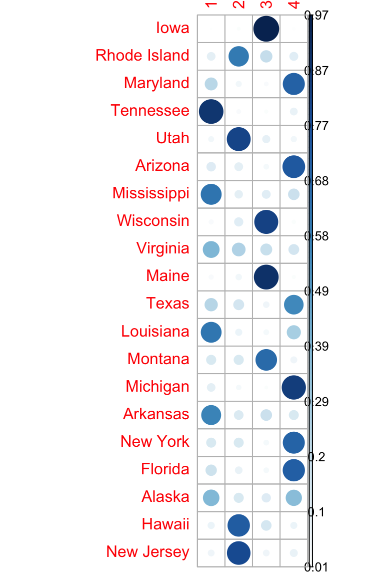
• membership: a matrix with the membership values of the data points to the clusters
• withinerror: the value of the objective function

Compute fuzzy c-means clustering

set.seed(123)

# Load the data
data("USArrests")
# Subset of USArrests
ss <- sample(1:50, 20)
df <- scale(USArrests[ss,])

# Compute fuzzy clustering
library(e1071)
cm <- cmeans(df, 4)
cm

## Fuzzy c-means clustering with 4 clusters
## 
## Cluster centers:
##   Murder Assault UrbanPop   Rape
## 1  0.857   0.338   -0.729  0.200
## 2 -0.731  -0.665    1.003 -0.333
## 3 -1.210  -1.248   -0.728 -1.153
## 4  0.629   0.970    0.501  0.865
## 
## Memberships:
##                    1      2      3       4
## Iowa         0.00916 0.0191 0.9658 0.00594
## Rhode Island 0.09885 0.5915 0.2050 0.10463
## Maryland     0.22786 0.0475 0.0273 0.69731
## Tennessee    0.87231 0.0286 0.0211 0.07801
## Utah         0.04446 0.8218 0.0844 0.04929
## Arizona      0.11876 0.1008 0.0399 0.74056
## Mississippi  0.62441 0.0931 0.1030 0.17952
## Wisconsin    0.03363 0.1110 0.8313 0.02403
## Virginia     0.39552 0.2570 0.1918 0.15573
## Maine        0.03433 0.0530 0.8915 0.02117
## Texas        0.24082 0.1595 0.0541 0.54557
## Louisiana    0.61799 0.0653 0.0419 0.27473
## Montana      0.13551 0.1366 0.6657 0.06215
## Michigan     0.09620 0.0371 0.0178 0.84890
## Arkansas     0.56529 0.1223 0.1805 0.13188
## New York     0.13194 0.1323 0.0416 0.69421
## Florida      0.17377 0.0749 0.0398 0.71155
## Alaska       0.38155 0.1354 0.1136 0.36947
## Hawaii       0.06662 0.7206 0.1487 0.06410
## New Jersey   0.05957 0.8009 0.0575 0.08206
## 
## Closest hard clustering:
##         Iowa Rhode Island     Maryland    Tennessee         Utah 
##            3            2            4            1            2 
##      Arizona  Mississippi    Wisconsin     Virginia        Maine 
##            4            1            3            1            3 
##        Texas    Louisiana      Montana     Michigan     Arkansas 
##            4            1            3            4            1 
##     New York      Florida       Alaska       Hawaii   New Jersey 
##            4            4            1            2            2 
## 
## Available components:
## [1] "centers"     "size"        "cluster"     "membership"  "iter"       
## [6] "withinerror" "call"

The different components can be extracted using the code below:

# Membership coefficient
head(cm$membership)

##                    1      2      3       4
## Iowa         0.00916 0.0191 0.9658 0.00594
## Rhode Island 0.09885 0.5915 0.2050 0.10463
## Maryland     0.22786 0.0475 0.0273 0.69731
## Tennessee    0.87231 0.0286 0.0211 0.07801
## Utah         0.04446 0.8218 0.0844 0.04929
## Arizona      0.11876 0.1008 0.0399 0.74056

# Visualize using corrplot
library(corrplot)
corrplot(cm$membership, is.corr = FALSE)

# Observation groups/clusters
cm$cluster

##         Iowa Rhode Island     Maryland    Tennessee         Utah 
##            3            2            4            1            2 
##      Arizona  Mississippi    Wisconsin     Virginia        Maine 
##            4            1            3            1            3 
##        Texas    Louisiana      Montana     Michigan     Arkansas 
##            4            1            3            4            1 
##     New York      Florida       Alaska       Hawaii   New Jersey 
##            4            4            1            2            2

Visualize clusters

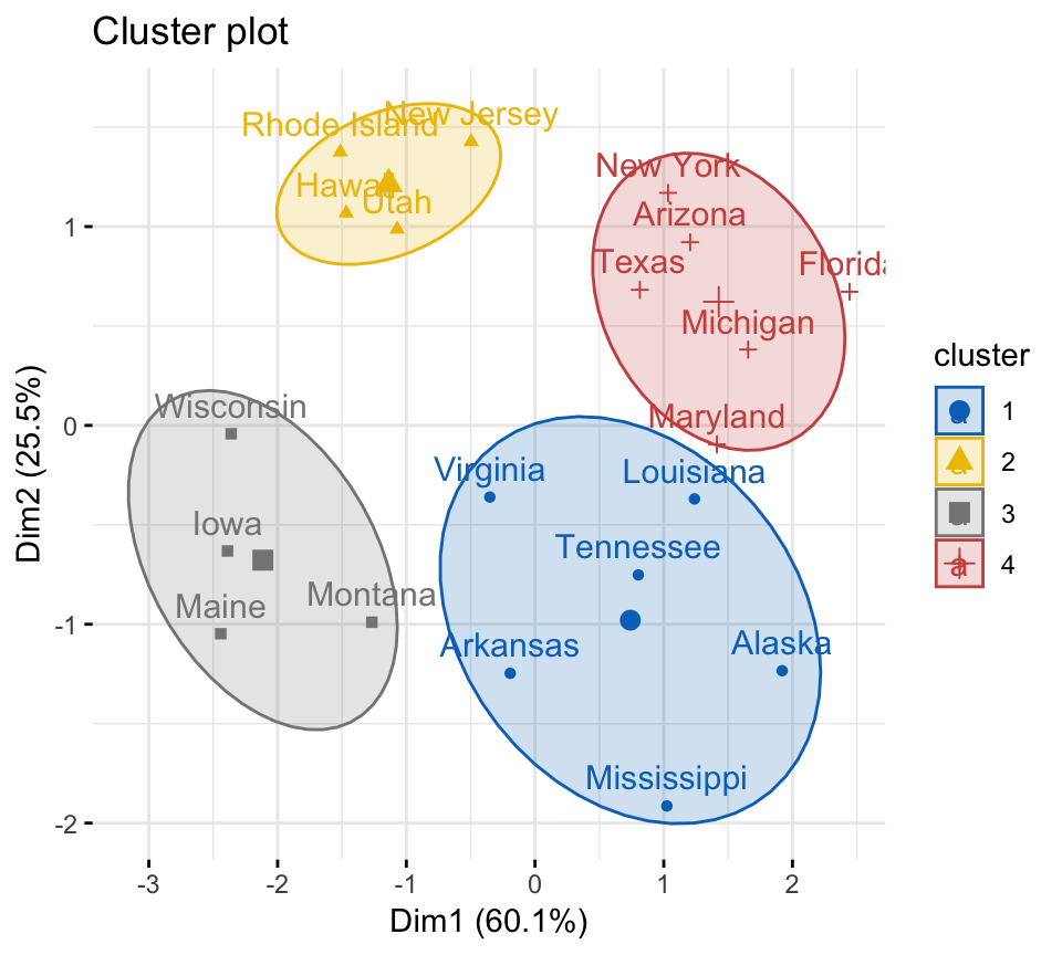
library(factoextra)
fviz_cluster(list(data = df, cluster=cm$cluster), 
             ellipse.type = "norm",
             ellipse.level = 0.68,
             palette = "jco",
             ggtheme = theme_minimal())