K-means clustering (MacQueen 1967) is one of the most commonly used unsupervised machine learning algorithm for partitioning a given data set into a set of k groups (i.e. k clusters), where k represents the number of groups pre-specified by the analyst. It classifies objects in multiple groups (i.e., clusters), such that objects within the same cluster are as similar as possible (i.e., high intra-class similarity), whereas objects from different clusters are as dissimilar as possible (i.e., low inter-class similarity). In k-means clustering, each cluster is represented by its center (i.e, centroid) which corresponds to the mean of points assigned to the cluster.
In this article, you will learn:
- The basic steps of k-means algorithm
- How to compute k-means in R software using practical examples
- Advantages and disavantages of k-means clustering
Contents:
Related Book
Practical Guide to Cluster Analysis in RK-means basic ideas
The basic idea behind k-means clustering consists of defining clusters so that the total intra-cluster variation (known as total within-cluster variation) is minimized.
There are several k-means algorithms available. The standard algorithm is the Hartigan-Wong algorithm (Hartigan and Wong 1979), which defines the total within-cluster variation as the sum of squared distances Euclidean distances between items and the corresponding centroid:
\[
W(C_k) = \sum\limits_{x_i \in C_k} (x_i - \mu_k)^2
\]
- \(x_i\) design a data point belonging to the cluster \(C_k\)
- \(\mu_k\) is the mean value of the points assigned to the cluster \(C_k\)
Each observation (\(x_i\)) is assigned to a given cluster such that the sum of squares (SS) distance of the observation to their assigned cluster centers \(\mu_k\) is a minimum.
We define the total within-cluster variation as follow:
\[
tot.withinss = \sum\limits_{k=1}^k W(C_k) = \sum\limits_{k=1}^k \sum\limits_{x_i \in C_k} (x_i - \mu_k)^2
\]
The total within-cluster sum of square measures the compactness (i.e goodness) of the clustering and we want it to be as small as possible.
K-means algorithm
The first step when using k-means clustering is to indicate the number of clusters (k) that will be generated in the final solution.
The algorithm starts by randomly selecting k objects from the data set to serve as the initial centers for the clusters. The selected objects are also known as cluster means or centroids.
Next, each of the remaining objects is assigned to it’s closest centroid, where closest is defined using the Euclidean distance between the object and the cluster mean. This step is called “cluster assignment step”. Note that, to use correlation distance, the data are input as z-scores.
After the assignment step, the algorithm computes the new mean value of each cluster. The term cluster “centroid update” is used to design this step. Now that the centers have been recalculated, every observation is checked again to see if it might be closer to a different cluster. All the objects are reassigned again using the updated cluster means.
The cluster assignment and centroid update steps are iteratively repeated until the cluster assignments stop changing (i.e until convergence is achieved). That is, the clusters formed in the current iteration are the same as those obtained in the previous iteration.
K-means algorithm can be summarized as follow:
- Specify the number of clusters (K) to be created (by the analyst)
- Select randomly k objects from the dataset as the initial cluster centers or means
- Assigns each observation to their closest centroid, based on the Euclidean distance between the object and the centroid
- For each of the k clusters update the cluster centroid by calculating the new mean values of all the data points in the cluster. The centoid of a Kth cluster is a vector of length p containing the means of all variables for the observations in the kth cluster; p is the number of variables.
- Iteratively minimize the total within sum of square. That is, iterate steps 3 and 4 until the cluster assignments stop changing or the maximum number of iterations is reached. By default, the R software uses 10 as the default value for the maximum number of iterations.
Computing k-means clustering in R
Data
We’ll use the demo data sets “USArrests”. The data should be prepared as described in chapter @ref(data-preparation-and-r-packages). The data must contains only continuous variables, as the k-means algorithm uses variable means. As we don’t want the k-means algorithm to depend to an arbitrary variable unit, we start by scaling the data using the R function scale() as follow:
data("USArrests")      # Loading the data set
df <- scale(USArrests) # Scaling the data

# View the firt 3 rows of the data
head(df, n = 3)
## Murder Assault UrbanPop Rape
## Alabama 1.2426 0.783 -0.521 -0.00342
## Alaska 0.5079 1.107 -1.212 2.48420
## Arizona 0.0716 1.479 0.999 1.04288Required R packages and functions
The standard R function for k-means clustering is kmeans() [stats package], which simplified format is as follow:
kmeans(x, centers, iter.max = 10, nstart = 1)- x: numeric matrix, numeric data frame or a numeric vector
- centers: Possible values are the number of clusters (k) or a set of initial (distinct) cluster centers. If a number, a random set of (distinct) rows in x is chosen as the initial centers.
- iter.max: The maximum number of iterations allowed. Default value is 10.
- nstart: The number of random starting partitions when centers is a number. Trying nstart > 1 is often recommended.
To create a beautiful graph of the clusters generated with the kmeans() function, will use the factoextra package.
- Installing factoextra package as:
install.packages("factoextra")- Loading factoextra:
library(factoextra)Estimating the optimal number of clusters
The k-means clustering requires the users to specify the number of clusters to be generated.
One fundamental question is: How to choose the right number of expected clusters (k)?
Different methods will be presented in the chapter “cluster evaluation and validation statistics”.
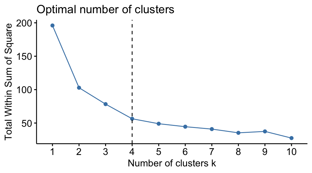
Here, we provide a simple solution. The idea is to compute k-means clustering using different values of clusters k. Next, the wss (within sum of square) is drawn according to the number of clusters. The location of a bend (knee) in the plot is generally considered as an indicator of the appropriate number of clusters.
The R function fviz_nbclust() [in factoextra package] provides a convenient solution to estimate the optimal number of clusters.
Claim Your Membership Now.

The plot above represents the variance within the clusters. It decreases as k increases, but it can be seen a bend (or “elbow”) at k = 4. This bend indicates that additional clusters beyond the fourth have little value.. In the next section, we’ll classify the observations into 4 clusters.
Computing k-means clustering
As k-means clustering algorithm starts with k randomly selected centroids, it’s always recommended to use the set.seed() function in order to set a seed for R’s random number generator. The aim is to make reproducible the results, so that the reader of this article will obtain exactly the same results as those shown below.
The R code below performs k-means clustering with k = 4:
# Compute k-means with k = 4
set.seed(123)
km.res <- kmeans(df, 4, nstart = 25)
As the final result of k-means clustering result is sensitive to the random starting assignments, we specify nstart = 25. This means that R will try 25 different random starting assignments and then select the best results corresponding to the one with the lowest within cluster variation. The default value of nstart in R is one. But, it’s strongly recommended to compute k-means clustering with a large value of nstart such as 25 or 50, in order to have a more stable result.
# Print the results
print(km.res)
## K-means clustering with 4 clusters of sizes 13, 16, 13, 8
##
## Cluster means:
## Murder Assault UrbanPop Rape
## 1 -0.962 -1.107 -0.930 -0.9668
## 2 -0.489 -0.383 0.576 -0.2617
## 3 0.695 1.039 0.723 1.2769
## 4 1.412 0.874 -0.815 0.0193
##
## Clustering vector:
## Alabama Alaska Arizona Arkansas California
## 4 3 3 4 3
## Colorado Connecticut Delaware Florida Georgia
## 3 2 2 3 4
## Hawaii Idaho Illinois Indiana Iowa
## 2 1 3 2 1
## Kansas Kentucky Louisiana Maine Maryland
## 2 1 4 1 3
## Massachusetts Michigan Minnesota Mississippi Missouri
## 2 3 1 4 3
## Montana Nebraska Nevada New Hampshire New Jersey
## 1 1 3 1 2
## New Mexico New York North Carolina North Dakota Ohio
## 3 3 4 1 2
## Oklahoma Oregon Pennsylvania Rhode Island South Carolina
## 2 2 2 2 4
## South Dakota Tennessee Texas Utah Vermont
## 1 4 3 2 1
## Virginia Washington West Virginia Wisconsin Wyoming
## 2 2 1 1 2
##
## Within cluster sum of squares by cluster:
## [1] 11.95 16.21 19.92 8.32
## (between_SS / total_SS = 71.2 %)
##
## Available components:
##
## [1] "cluster" "centers" "totss" "withinss"
## [5] "tot.withinss" "betweenss" "size" "iter"
## [9] "ifault"The printed output displays:
- the cluster means or centers: a matrix, which rows are cluster number (1 to 4) and columns are variables
- the clustering vector: A vector of integers (from 1:k) indicating the cluster to which each point is allocated
It’s possible to compute the mean of each variables by clusters using the original data:
aggregate(USArrests, by=list(cluster=km.res$cluster), mean)## cluster Murder Assault UrbanPop Rape
## 1 1 3.60 78.5 52.1 12.2
## 2 2 5.66 138.9 73.9 18.8
## 3 3 10.82 257.4 76.0 33.2
## 4 4 13.94 243.6 53.8 21.4If you want to add the point classifications to the original data, use this:
dd <- cbind(USArrests, cluster = km.res$cluster)
head(dd)
## Murder Assault UrbanPop Rape cluster
## Alabama 13.2 236 58 21.2 4
## Alaska 10.0 263 48 44.5 3
## Arizona 8.1 294 80 31.0 3
## Arkansas 8.8 190 50 19.5 4
## California 9.0 276 91 40.6 3
## Colorado 7.9 204 78 38.7 3Accessing to the results of kmeans() function
kmeans() function returns a list of components, including:
- cluster: A vector of integers (from 1:k) indicating the cluster to which each point is allocated
- centers: A matrix of cluster centers (cluster means)
- totss: The total sum of squares (TSS), i.e \(\sum{(x_i - \bar{x})^2}\). TSS measures the total variance in the data.
- withinss: Vector of within-cluster sum of squares, one component per cluster
- tot.withinss: Total within-cluster sum of squares, i.e. \(sum(withinss)\)
- betweenss: The between-cluster sum of squares, i.e. \(totss - tot.withinss\)
- size: The number of observations in each cluster
These components can be accessed as follow:
# Cluster number for each of the observations
km.res$cluster
head(km.res$cluster, 4)## Alabama Alaska Arizona Arkansas
## 4 3 3 4…..
# Cluster size
km.res$size
## [1] 13 16 13 8# Cluster means
km.res$centers## Murder Assault UrbanPop Rape
## 1 -0.962 -1.107 -0.930 -0.9668
## 2 -0.489 -0.383 0.576 -0.2617
## 3 0.695 1.039 0.723 1.2769
## 4 1.412 0.874 -0.815 0.0193Visualizing k-means clusters
It is a good idea to plot the cluster results. These can be used to assess the choice of the number of clusters as well as comparing two different cluster analyses.
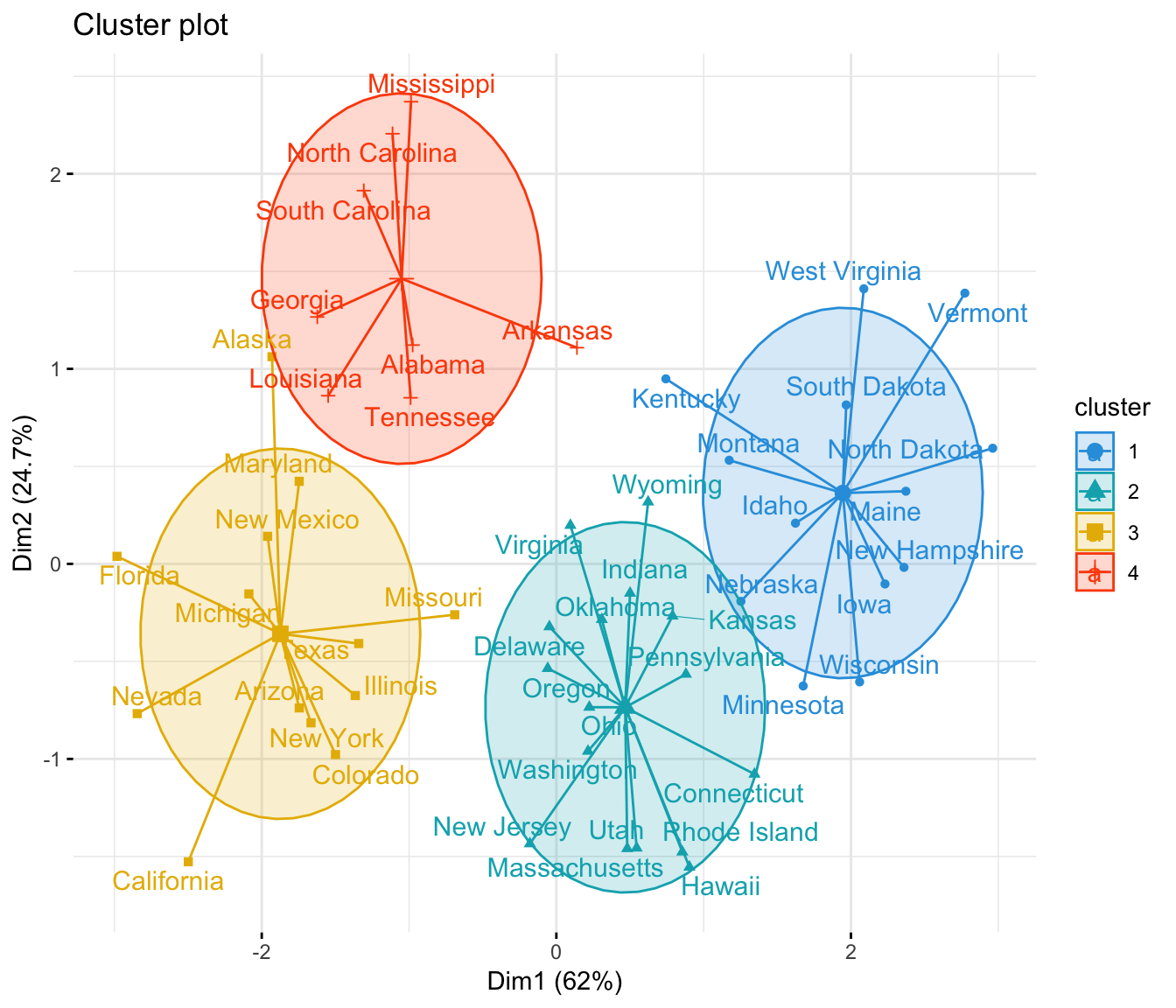
Now, we want to visualize the data in a scatter plot with coloring each data point according to its cluster assignment.
The problem is that the data contains more than 2 variables and the question is what variables to choose for the xy scatter plot.
A solution is to reduce the number of dimensions by applying a dimensionality reduction algorithm, such as Principal Component Analysis (PCA), that operates on the four variables and outputs two new variables (that represent the original variables) that you can use to do the plot.
In other words, if we have a multi-dimensional data set, a solution is to perform Principal Component Analysis (PCA) and to plot data points according to the first two principal components coordinates.
The function fviz_cluster() [factoextra package] can be used to easily visualize k-means clusters. It takes k-means results and the original data as arguments. In the resulting plot, observations are represented by points, using principal components if the number of variables is greater than 2. It’s also possible to draw concentration ellipse around each cluster.
Claim Your Membership Now.

K-means clustering advantages and disadvantages
K-means clustering is very simple and fast algorithm. It can efficiently deal with very large data sets. However there are some weaknesses, including:
- It assumes prior knowledge of the data and requires the analyst to choose the appropriate number of cluster (k) in advance
- The final results obtained is sensitive to the initial random selection of cluster centers. Why is it a problem? Because, for every different run of the algorithm on the same dataset, you may choose different set of initial centers. This may lead to different clustering results on different runs of the algorithm.
- It’s sensitive to outliers.
- If you rearrange your data, it’s very possible that you’ll get a different solution every time you change the ordering of your data.
Possible solutions to these weaknesses, include:
- Solution to issue 1: Compute k-means for a range of k values, for example by varying k between 2 and 10. Then, choose the best k by comparing the clustering results obtained for the different k values.
- Solution to issue 2: Compute K-means algorithm several times with different initial cluster centers. The run with the lowest total within-cluster sum of square is selected as the final clustering solution.
- To avoid distortions caused by excessive outliers, it’s possible to use PAM algorithm, which is less sensitive to outliers.
Alternative to k-means clustering
A robust alternative to k-means is PAM, which is based on medoids. As discussed in the next chapter, the PAM clustering can be computed using the function pam() [cluster package]. The function pamk( ) [fpc package] is a wrapper for PAM that also prints the suggested number of clusters based on optimum average silhouette width.
Summary
K-means clustering can be used to classify observations into k groups, based on their similarity. Each group is represented by the mean value of points in the group, known as the cluster centroid.
K-means algorithm requires users to specify the number of cluster to generate. The R function kmeans() [stats package] can be used to compute k-means algorithm. The simplified format is kmeans(x, centers), where “x” is the data and centers is the number of clusters to be produced.
After, computing k-means clustering, the R function fviz_cluster() [factoextra package] can be used to visualize the results. The format is fviz_cluster(km.res, data), where km.res is k-means results and data corresponds to the original data sets.
References
Hartigan, JA, and MA Wong. 1979. “Algorithm AS 136: A K-means clustering algorithm.” Applied Statistics. Royal Statistical Society, 100–108.
MacQueen, J. 1967. “Some Methods for Classification and Analysis of Multivariate Observations.” In Proceedings of the Fifth Berkeley Symposium on Mathematical Statistics and Probability, Volume 1: Statistics, 281–97. Berkeley, Calif.: University of California Press. http://projecteuclid.org:443/euclid.bsmsp/1200512992.
Recommended for you
This section contains best data science and self-development resources to help you on your path.
Books - Data Science
Our Books
- Practical Guide to Cluster Analysis in R by A. Kassambara (Datanovia)
- Practical Guide To Principal Component Methods in R by A. Kassambara (Datanovia)
- Machine Learning Essentials: Practical Guide in R by A. Kassambara (Datanovia)
- R Graphics Essentials for Great Data Visualization by A. Kassambara (Datanovia)
- GGPlot2 Essentials for Great Data Visualization in R by A. Kassambara (Datanovia)
- Network Analysis and Visualization in R by A. Kassambara (Datanovia)
- Practical Statistics in R for Comparing Groups: Numerical Variables by A. Kassambara (Datanovia)
- Inter-Rater Reliability Essentials: Practical Guide in R by A. Kassambara (Datanovia)
Others
- R for Data Science: Import, Tidy, Transform, Visualize, and Model Data by Hadley Wickham & Garrett Grolemund
- Hands-On Machine Learning with Scikit-Learn, Keras, and TensorFlow: Concepts, Tools, and Techniques to Build Intelligent Systems by Aurelien Géron
- Practical Statistics for Data Scientists: 50 Essential Concepts by Peter Bruce & Andrew Bruce
- Hands-On Programming with R: Write Your Own Functions And Simulations by Garrett Grolemund & Hadley Wickham
- An Introduction to Statistical Learning: with Applications in R by Gareth James et al.
- Deep Learning with R by François Chollet & J.J. Allaire
- Deep Learning with Python by François Chollet


how we can get data
The demo data used in this tutorial is available in the default installation of R. Juste type data(“USArrests”)