Advanced Clustering

Concept of model-based clustering

In model-based clustering, the data is considered as coming from a mixture of density.

Each component (i.e. cluster) k is modeled by the normal or Gaussian distribution which is characterized by the parameters:

• \(\mu_k\): mean vector,
• \(\sum_k\): covariance matrix,
• An associated probability in the mixture. Each point has a probability of belonging to each cluster.

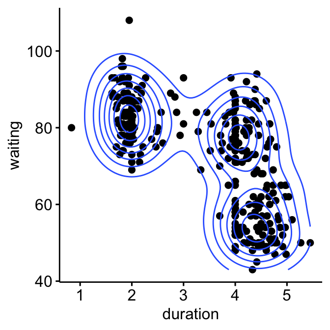
For example, consider the “old faithful geyser data” [in MASS R package], which can be illustrated as follow using the ggpubr R package:

# Load the data
library("MASS")
data("geyser")

# Scatter plot
library("ggpubr")
ggscatter(geyser, x = "duration", y = "waiting")+
  geom_density2d() # Add 2D density

The plot above suggests at least 3 clusters in the mixture. The shape of each of the 3 clusters appears to be approximately elliptical suggesting three bivariate normal distributions. As the 3 ellipses seems to be similar in terms of volume, shape and orientation, we might anticipate that the three components of this mixture might have homogeneous covariance matrices.

Estimating model parameters

The model parameters can be estimated using the Expectation-Maximization (EM) algorithm initialized by hierarchical model-based clustering. Each cluster k is centered at the means \(\mu_k\), with increased density for points near the mean.

Geometric features (shape, volume, orientation) of each cluster are determined by the covariance matrix \(\sum_k\).

Different possible parameterizations of \(\sum_k\) are available in the R package mclust (see ?mclustModelNames).

The available model options, in mclust package, are represented by identifiers including: EII, VII, EEI, VEI, EVI, VVI, EEE, EEV, VEV and VVV.

The first identifier refers to volume, the second to shape and the third to orientation. E stands for “equal”, V for “variable” and I for “coordinate axes”.

For example:

• EVI denotes a model in which the volumes of all clusters are equal (E), the shapes of the clusters may vary (V), and the orientation is the identity (I) or “coordinate axes.
• EEE means that the clusters have the same volume, shape and orientation in p-dimensional space.
• VEI means that the clusters have variable volume, the same shape and orientation equal to coordinate axes.

Choosing the best model

The Mclust package uses maximum likelihood to fit all these models, with different covariance matrix parameterizations, for a range of k components.

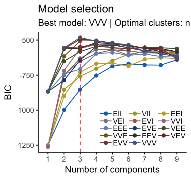
The best model is selected using the Bayesian Information Criterion or BIC. A large BIC score indicates strong evidence for the corresponding model.

Computing model-based clustering in R

We start by installing the mclust package as follow: install.packages(“mclust”)

Here, we illustrate model-based clustering on the diabetes data set [mclust package] giving three measurements and the diagnosis for 145 subjects described as follow:

library("mclust")
data("diabetes")
head(diabetes, 3)

##    class glucose insulin sspg
## 1 Normal      80     356  124
## 2 Normal      97     289  117
## 3 Normal     105     319  143

• class: the diagnosis: normal, chemically diabetic, and overtly diabetic. Excluded from the cluster analysis.
• glucose: plasma glucose response to oral glucose
• insulin: plasma insulin response to oral glucose
• sspg: steady-state plasma glucose (measures insulin resistance)

Model-based clustering can be computed using the function Mclust() as follow:

library(mclust)
df <- scale(diabetes[, -1]) # Standardize the data
mc <- Mclust(df)            # Model-based-clustering

summary(mc)                 # Print a summary

## ----------------------------------------------------
## Gaussian finite mixture model fitted by EM algorithm 
## ----------------------------------------------------
## 
## Mclust VVV (ellipsoidal, varying volume, shape, and orientation) model with 3 components:
## 
##  log.likelihood   n df  BIC  ICL
##            -169 145 29 -483 -501
## 
## Clustering table:
##  1  2  3 
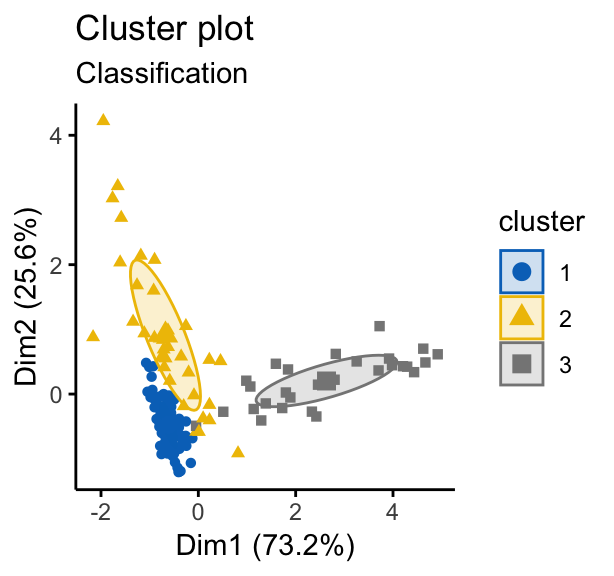
## 81 36 28

For this data, it can be seen that model-based clustering selected a model with three components (i.e. clusters). The optimal selected model name is VVV model. That is the three components are ellipsoidal with varying volume, shape, and orientation. The summary contains also the clustering table specifying the number of observations in each clusters.

You can access to the results as follow:

mc$modelName                # Optimal selected model ==> "VVV"
mc$G                        # Optimal number of cluster => 3
head(mc$z, 30)              # Probality to belong to a given cluster
head(mc$classification, 30) # Cluster assignement of each observation

Visualizing model-based clustering

Model-based clustering results can be drawn using the base function plot.Mclust() [in mclust package]. Here we’ll use the function fviz_mclust() [in factoextra package] to create beautiful plots based on ggplot2.

In the situation, where the data contain more than two variables, fviz_mclust() uses a principal component analysis to reduce the dimensionnality of the data. The first two principal components are used to produce a scatter plot of the data. However, if you want to plot the data using only two variables of interest, let say here c(“insulin”, “sspg”), you can specify that in the fviz_mclust() function using the argument choose.vars = c(“insulin”, “sspg”).

library(factoextra)
# BIC values used for choosing the number of clusters
fviz_mclust(mc, "BIC", palette = "jco")
# Classification: plot showing the clustering
fviz_mclust(mc, "classification", geom = "point", 
            pointsize = 1.5, palette = "jco")
# Classification uncertainty
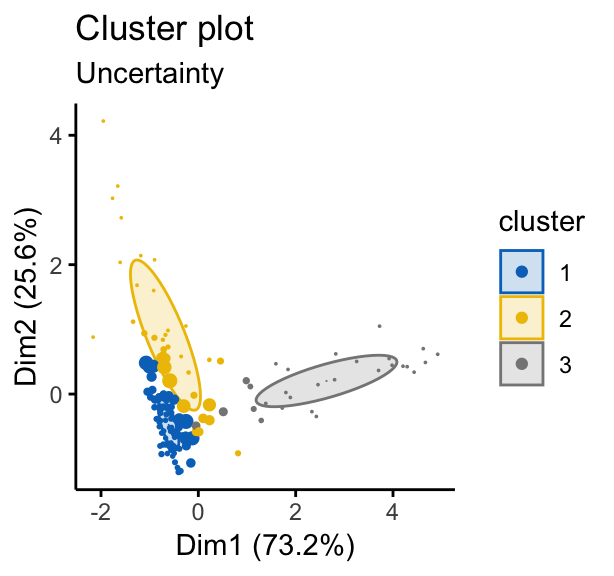
fviz_mclust(mc, "uncertainty", palette = "jco")

Note that, in the uncertainty plot, larger symbols indicate the more uncertain observations.

References

Fraley, Chris, and Adrian E Raftery. 2002. “Model-Based Clustering, Discriminant Analysis, and Density Estimation.” Journal of the American Statistical Association 97 (458): 611–31.
Fraley, Chris, Adrian E. Raftery, T. Brendan Murphy, and Luca Scrucca. 2012. “Mclust Version 4 for R: Normal Mixture Modeling for Model-Based Clustering, Classification, and Density Estimation.” Technical Report No. 597, Department of Statistics, University of Washington. https://www.stat.washington.edu/research/reports/2012/tr597.pdf.
Recommended for you
This section contains best data science and self-development resources to help you on your path.
Books - Data Science
Our Books
- Practical Guide to Cluster Analysis in R by A. Kassambara (Datanovia)
- Practical Guide To Principal Component Methods in R by A. Kassambara (Datanovia)
- Machine Learning Essentials: Practical Guide in R by A. Kassambara (Datanovia)
- R Graphics Essentials for Great Data Visualization by A. Kassambara (Datanovia)
- GGPlot2 Essentials for Great Data Visualization in R by A. Kassambara (Datanovia)
- Network Analysis and Visualization in R by A. Kassambara (Datanovia)
- Practical Statistics in R for Comparing Groups: Numerical Variables by A. Kassambara (Datanovia)
- Inter-Rater Reliability Essentials: Practical Guide in R by A. Kassambara (Datanovia)
Others
- R for Data Science: Import, Tidy, Transform, Visualize, and Model Data by Hadley Wickham & Garrett Grolemund
- Hands-On Machine Learning with Scikit-Learn, Keras, and TensorFlow: Concepts, Tools, and Techniques to Build Intelligent Systems by Aurelien Géron
- Practical Statistics for Data Scientists: 50 Essential Concepts by Peter Bruce & Andrew Bruce
- Hands-On Programming with R: Write Your Own Functions And Simulations by Garrett Grolemund & Hadley Wickham
- An Introduction to Statistical Learning: with Applications in R by Gareth James et al.
- Deep Learning with R by François Chollet & J.J. Allaire
- Deep Learning with Python by François Chollet
MERCI BEAUCOUP
THANK YOU SO MUCH
FOR THE COLORS YOU PUT ON THE DATA TO MAKE THEM
REALLY TALK TO US
I ENJOY PLOTTING AND MODELLING AND CLUSTRING
LEARNING FROM YOU HOW TO DO A BEAUTIFULL DATA ANALYSIS
THANK YOU SIR TO SHARE THIS JOY
WISH YOU THE BEST
REGARDS
Hi Chafia,
Thank you very much for the feedback.
These kind of appreciations really help and motivate us to perform well and deliver better contents forever.
Thank you again.
Best regards
Hi Kas,
Thanks for sharing, like Chafia, I agree that this is very helpful.
I have .a quick question about the intuition around scale and using a distance matrix (or method). I find that in certain instance, data is scaled and in others, a distance method such as Bray Curtis or Jaccardi is used. Am referring to microbiome studies. What are your thoughts?
Thanks,
Hi San Emmanuel,
Thank you for your feedback!
The choice of the (dis)simality metric shoud be based on the research question and the type of dataset.
For example, Euclidian distance is best for variables with continuous data while Bray Curtis is best for categorical or binary data.
Particularly for continuous data it is expected that all variables are in the “same” scale and with the “same” distribution. So if your variables are not, you will need to standardize or normalize them.
If You want to reflect ecological differences, then Bray-Curtis will do a much better job, since it used to quantify the compositional dissimilarity between two different sites, based on counts at each site.
The Bray–Curtis dissimilarity is often erroneously called a distance. It is not a distance since it does not satisfy triangle inequality, and should always be called a dissimilarity to avoid confusion.
The use of Euclidean (metric distance) and Bray-Curtis (semi metric) depends on your data and the way you want to handle it. Metric distances comply with the triangle inequality criterion (the sum of two sides of a triangle equal must be greatet or equal than the other side) while semi metric don’t.
This is particularly relevant when zeros are not true absences (eg when you sample species from a site, you’ll never know for sure if the species is truly absent or you failed to sample it but is present, or in your case metals).
This is very important because if your zeros aren’t true absences and you use Euclidean distance, the dissimilarities among sites won’t be a good description of your data, that is, two sites with a bunch of shared zeros will be more similar to each other this two sites with a few shared observations. This is why, when dealing with composition data, it is more appropriate to use Bray-Curtis over Euclidean distance.
See also:
– Clustering Distance Measures, https://www.datanovia.com/en/lessons/clustering-distance-measures/
Thank you SO much for this to-the-point, beautiful post!
It really helped me with my first steps.
I rarely come across such easy-to-understand and useful post in this topic that helps beginners too!
Do you think using this mclust approach is adequate for a dataset that contains only X and Y coordinates of objects? I mean it works beautifully, but is it the proper way? I can get very lost in all the possible spatial clustering methods. I was also looking at DBSCAN but mclust gives much better plots (I think).
Thanks again:)
Teadora
Thank you for your positive feedback, highly appreciated!
Yes you can use model based clustering on two-dimensional data sets:
# Data preparation
data("geyser", package = "MASS")
df <- scale(geyser)
# Model baseq clusering