One-Way MANOVA in R: The Ultimate Practical Guide

One-Way MANOVA in R

20 mins

The Multivariate Analysis Of Variance (MANOVA) is an ANOVA with two or more continuous outcome (or response) variables.

The one-way MANOVA tests simultaneously statistical differences for multiple response variables by one grouping variables.

For example, we may conduct an experiment where we give two treatments (A and B) to two groups of mice, and we are interested in the weight and height of mice. In that case, the weight and height of mice are our outcome (or dependent) variables, and our hypothesis is that both together are affected by the difference in treatment. A multivariate analysis of variance could be used to test this hypothesis.

The procedure of MANOVA can be summarized as follow:

Create a new composite variable that is a linear combination of all the response variables.
Compare the mean values of this new variable between groups.

This article describes how to compute one-way MANOVA in R.

Note that, MANOVA is appropriate in experimental situations, where we have several outcome (dependent) variables which all measure different aspects of some cohesive theme. For example, several exam scores to have a measure of overall academic performance.

Contents:

Related Book

Practical Statistics in R II - Comparing Groups: Numerical Variables

Prerequisites

Make sure that you have installed the following R packages:

tidyverse for data manipulation and visualization
ggpubr for creating easily publication ready plots
rstatix for easy pipe-friendly statistical analyses
car for MANOVA analyses
broom for printing a nice summary of statistical tests as data frames
datarium contains required data sets for this chapter

Start by loading the following R packages:

library(tidyverse)
library(ggpubr)
library(rstatix)
library(car)
library(broom)

Data preparation

We’ll use the built-in R dataset iris. Select columns of interest:

iris2 <- iris %>%
  select(Sepal.Length, Petal.Length, Species) %>%
  add_column(id = 1:nrow(iris), .before = 1)
head(iris2)

##   id Sepal.Length Petal.Length Species
## 1  1          5.1          1.4  setosa
## 2  2          4.9          1.4  setosa
## 3  3          4.7          1.3  setosa
## 4  4          4.6          1.5  setosa
## 5  5          5.0          1.4  setosa
## 6  6          5.4          1.7  setosa

Visualization

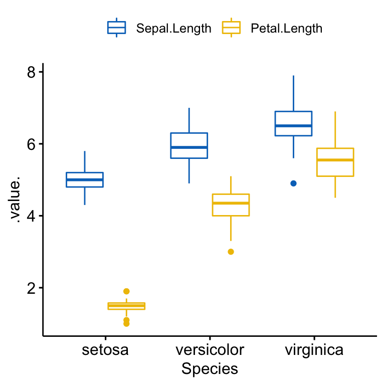
The R code below creates a merged box plots of Sepal.Length and Petal.Length by Species groups.

ggboxplot(
  iris2, x = "Species", y = c("Sepal.Length", "Petal.Length"), 
  merge = TRUE, palette = "jco"
  )

Summary statistics

Compute summary statistics (mean, SD) by groups for each outcome variable:

iris2 %>%
  group_by(Species) %>%
  get_summary_stats(Sepal.Length, Petal.Length, type = "mean_sd")

## # A tibble: 6 x 5
##   Species    variable         n  mean    sd
##   <fct>      <chr>        <dbl> <dbl> <dbl>
## 1 setosa     Petal.Length    50  1.46 0.174
## 2 setosa     Sepal.Length    50  5.01 0.352
## 3 versicolor Petal.Length    50  4.26 0.47 
## 4 versicolor Sepal.Length    50  5.94 0.516
## 5 virginica  Petal.Length    50  5.55 0.552
## 6 virginica  Sepal.Length    50  6.59 0.636

Assumptions and preleminary tests

MANOVA makes the following assumptions about the data:

Adequate sample size. Rule of thumb: the n in each cell > the number of outcome variables.
Independence of the observations. Each subject should belong to only one group. There is no relationship between the observations in each group. Having repeated measures for the same participants is not allowed. The selection of the sample should be completely random.
Absense of univariate or multivariate outliers.
Multivariate normality. The R function mshapiro_test( )[in the rstatix package] can be used to perform the Shapiro-Wilk test for multivariate normality.
Absence of multicollinearity. The dependent (outcome) variables cannot be too correlated to each other. No correlation should be above r = 0.90 [Tabachnick and Fidell (2012)}.
Linearity between all outcome variables for each group.
Homogeneity of variances. The Levene’s test can be used to test the equality of variances between groups. Non-significant values of Levene’s test indicate equal variance between groups.
Homogeneity of variance-covariance matrices. The Box’s M Test can be used to check the equality of covariance between the groups. This is the equivalent of a multivariate homogeneity of variance. This test is considered as highly sensitive. Therefore, significance for this test is determined at alpha = 0.001.

Check sample size assumption

iris2 %>%
  group_by(Species) %>%
  summarise(N = n())

## # A tibble: 3 x 2
##   Species        N
##   <fct>      <int>
## 1 setosa        50
## 2 versicolor    50
## 3 virginica     50

As the table above shows 50 observations per group, the assumption of adequate sample size is satisfied.

Identify univariate outliers

Univariate outliers can be easily identified using box plot methods, implemented in the R function identify_outliers() [rstatix package].

Group the data by Species and then, identify outliers in the Sepal.Length variable:

iris2 %>%
  group_by(Species) %>%
  identify_outliers(Sepal.Length)

## # A tibble: 1 x 6
##   Species      id Sepal.Length Petal.Length is.outlier is.extreme
##   <fct>     <int>        <dbl>        <dbl> <lgl>      <lgl>     
## 1 virginica   107          4.9          4.5 TRUE       FALSE

Group the data by Species and then, identify outliers in the Petal.Length variable:

iris2 %>%
  group_by(Species) %>%
  identify_outliers(Petal.Length)

## # A tibble: 5 x 6
##   Species       id Sepal.Length Petal.Length is.outlier is.extreme
##   <fct>      <int>        <dbl>        <dbl> <lgl>      <lgl>     
## 1 setosa        14          4.3          1.1 TRUE       FALSE     
## 2 setosa        23          4.6          1   TRUE       FALSE     
## 3 setosa        25          4.8          1.9 TRUE       FALSE     
## 4 setosa        45          5.1          1.9 TRUE       FALSE     
## 5 versicolor    99          5.1          3   TRUE       FALSE

There were no univariate extreme outliers in the Sepal.Length and Petal.length variable, as assessed by box plot methods.

Note that, in the situation where you have extreme outliers, this can be due to: 1) data entry errors, measurement errors or unusual values.

Yo can include the outlier in the analysis anyway if you do not believe the result will be substantially affected. This can be evaluated by comparing the result of the MANOVA with and without the outlier.

Remember to report in your written results section any decisions you make regarding any outliers you find.

Detect multivariate outliers

Multivariate outliers are data points that have an unusual combination of values on the outcome (or dependent) variables.

In MANOVA setting, the Mahalanobis distance is generally used to detect multivariate outliers. The distance tells us how far an observation is from the center of the cloud, taking into account the shape (covariance) of the cloud as well.

The function mahalanobis_distance() [rstatix package] can be easily used to compute the Mahalanobis distance and to flag multivariate outliers. Read more in the documentation of the function.

This metric needs to be calculated by groups:

# Compute distance by groups and filter outliers
# Use -id to omit the id column in the computation
iris2 %>%
 group_by(Species) %>%
 mahalanobis_distance(-id) %>%
 filter(is.outlier == TRUE) %>%
  as.data.frame()

## [1] id           Sepal.Length Petal.Length mahal.dist   is.outlier  
## <0 rows> (or 0-length row.names)

There were no multivariate outliers in the data, as assessed by Mahalanobis distance (p > 0.001).

If you have multivariate outliers, you could consider running MANOVA before and after removing the outlier to check whether or not their presence alter the results. You should report your final decision.

Check univariate normality assumption

The normality assumption can be checked by computing Shapiro-Wilk test for each outcome variable at each level of the grouping variable. If the data is normally distributed, the p-value should be greater than 0.05.

iris2 %>%
  group_by(Species) %>%
  shapiro_test(Sepal.Length, Petal.Length) %>%
  arrange(variable)

## # A tibble: 6 x 4
##   Species    variable     statistic      p
##   <fct>      <chr>            <dbl>  <dbl>
## 1 setosa     Petal.Length     0.955 0.0548
## 2 versicolor Petal.Length     0.966 0.158 
## 3 virginica  Petal.Length     0.962 0.110 
## 4 setosa     Sepal.Length     0.978 0.460 
## 5 versicolor Sepal.Length     0.978 0.465 
## 6 virginica  Sepal.Length     0.971 0.258

Sepal.Length and Petal.length were normally distributed for each Species groups, as assessed by Shapiro-Wilk’s test (p > 0.05).

You can also create QQ plot for each group. QQ plot draws the correlation between a given data and the normal distribution.

# QQ plot of Sepal.Length
ggqqplot(iris2, "Sepal.Length", facet.by = "Species",
         ylab = "Sepal Length", ggtheme = theme_bw())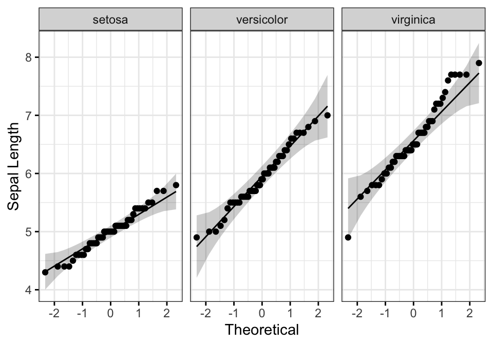

# QQ plot of Petal.Length
ggqqplot(iris2, "Petal.Length", facet.by = "Species",
         ylab = "Petal Length", ggtheme = theme_bw())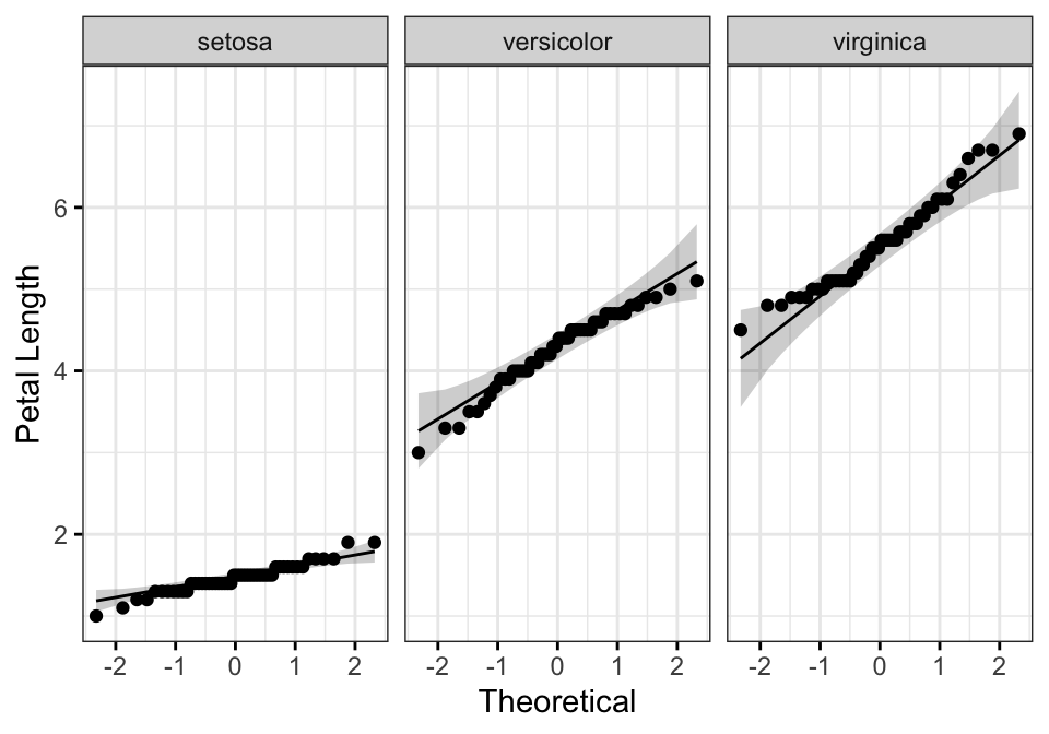

All the points fall approximately along the reference line, for each group. So we can assume normality of the data.

Note that, if your sample size is greater than 50, the normal QQ plot is preferred because at larger sample sizes the Shapiro-Wilk test becomes very sensitive even to a minor deviation from normality.

In the situation where the assumptions are not met, you could consider running MANOVA on the data after transforming the outcome variables. You can also perform the test regardless as MANOVA is fairly robust to deviations from normality.

Multivariate normality

iris2 %>%
  select(Sepal.Length, Petal.Length) %>%
  mshapiro_test()

## # A tibble: 1 x 2
##   statistic p.value
##       <dbl>   <dbl>
## 1     0.995   0.855

The test is not significant (p > 0.05), so we can assume multivariate normality.

Identify multicollinearity

Ideally the correlation between the outcome variables should be moderate, not too high. A correlation above 0.9 is an indication of multicollinearity, which is problematic for MANOVA.

In other hand, if the correlation is too low, you should consider running separate one-way ANOVA for each outcome variable.

Compute pairwise Pearson correlation coefficients between the outcome variable. In the following R code, we’ll use the function cor_test() [rstatix package]. If you have more than two outcome variables, consider using the function cor_mat():

iris2 %>% cor_test(Sepal.Length, Petal.Length)

## # A tibble: 1 x 8
##   var1         var2           cor statistic        p conf.low conf.high method 
##   <chr>        <chr>        <dbl>     <dbl>    <dbl>    <dbl>     <dbl> <chr>  
## 1 Sepal.Length Petal.Length  0.87      21.6 1.04e-47    0.827     0.906 Pearson

There was no multicollinearity, as assessed by Pearson correlation (r = 0.87, p < 0.0001).

In the situation, where you have multicollinearity, you could consider removing one of the outcome variables that is highly correlated.

Check linearity assumption

The pairwise relationship between the outcome variables should be linear for each group. This can be checked visually by creating a scatter plot matrix using the R function ggpairs() [GGally package]. In our example, we have only one pair:

# Create a scatterplot matrix by group
library(GGally)
results <- iris2 %>%
  select(Sepal.Length, Petal.Length, Species) %>%
  group_by(Species) %>%
  doo(~ggpairs(.) + theme_bw(), result = "plots")
results

## # A tibble: 3 x 2
##   Species    plots 
##   <fct>      <list>
## 1 setosa     <gg>  
## 2 versicolor <gg>  
## 3 virginica  <gg>

# Show the plots
results$plots

## [[1]]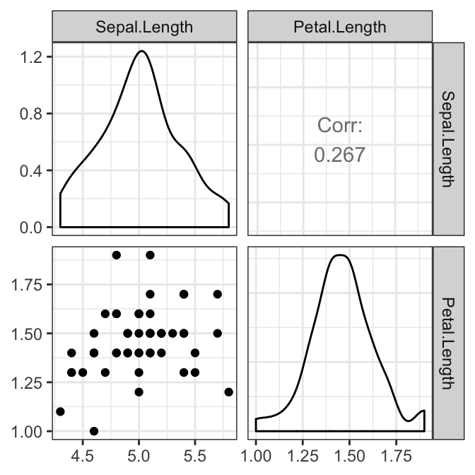

## 
## [[2]]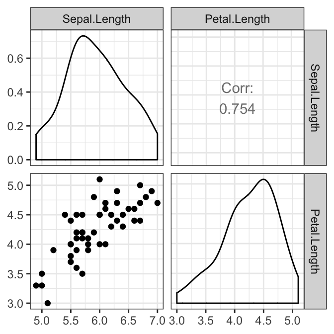

## 
## [[3]]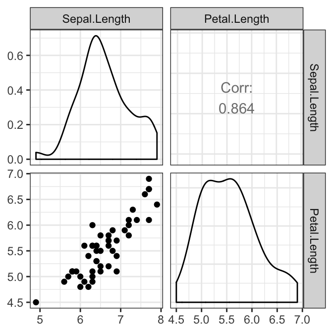

There was a linear relationship between Sepal.Length and Petal.Length in each Species group, as assessed by scatter plot.

In the situation, where you detect non-linear relationships, You can:

transform or remove the concerned outcome variables;
run the analysis anyway. You will loss some power.

Check the homogeneity of covariances assumption

This can be evaluated using the Box’s M-test implemented in the rstatix package.

box_m(iris2[, c("Sepal.Length", "Petal.Length")], iris2$Species)

## # A tibble: 1 x 4
##   statistic  p.value parameter method                                             
##       <dbl>    <dbl>     <dbl> <chr>                                              
## 1      58.4 9.62e-11         6 Box's M-test for Homogeneity of Covariance Matrices

The test is statistically significant (i.e., p < 0.001), so the data have violated the assumption of homogeneity of variance-covariance matrices.

Note that, if you have balanced design (i.e., groups with similar sizes), you don’t need to worry too much about violation of the homogeneity of variances-covariance matrices and you can continue your analysis.

However, having an unbalanced design is problematic. Possible solutions include: 1) transforming the dependent variables; 2) running the test anyway, but using Pillai’s multivariate statistic instead of Wilks’ statistic.

Check the homogneity of variance assumption

For each of the outcome variables, the one-way MANOVA assumes that there are equal variances between groups. This can be checked using the Levene’s test of equality of variances. Key R function: levene_test() [rstatix package].

Procedure:

Gather the outcome variables into key-value pairs
Group by variable
Compute the Levene’s test

iris2 %>% 
  gather(key = "variable", value = "value", Sepal.Length, Petal.Length) %>%
  group_by(variable) %>%
  levene_test(value ~ Species)

## # A tibble: 2 x 5
##   variable       df1   df2 statistic            p
##   <chr>        <int> <int>     <dbl>        <dbl>
## 1 Petal.Length     2   147     19.5  0.0000000313
## 2 Sepal.Length     2   147      6.35 0.00226

The Levene’s test is significant (p < 0.05), so there was no homogeneity of variances.

Note that, if you do not have homogeneity of variances, you can try to transform the outcome (dependent) variable to correct for the unequal variances.

Alternatively, you can continue, but accept a lower level of statistical significance (alpha level) for your MANOVA result. Additionally, any follow-up univariate ANOVAs will need to be corrected for this violation (i.e., you will need to use different post-hoc tests).

Computation

There are four different types of multivariate statistics that can be used for computing MANOVA. These are: “Pillai”, “Wilks”, “Hotelling-Lawley”, or “Roy”.

The most commonly recommended multivariate statistic to use is Wilks’ Lambda.

However, Pillai’s Trace is more robust and is recommended when you have unbalanced design and also have a statistically significant Box’s M result (as in our example, see previous section).

Note that, “Pillai” is the default in the R Manova() function [car package].

Compute MANOVA:

model <- lm(cbind(Sepal.Length, Petal.Length) ~ Species, iris2)
Manova(model, test.statistic = "Pillai")

## 
## Type II MANOVA Tests: Pillai test statistic
##         Df test stat approx F num Df den Df Pr(>F)    
## Species  2     0.989     71.8      4    294 <2e-16 ***
## ---
## Signif. codes:  0 '***' 0.001 '**' 0.01 '*' 0.05 '.' 0.1 ' ' 1

There was a statistically significant difference between the Species on the combined dependent variables (Sepal.Length and Petal.Length), F(4, 294) = 71.829, p < 0.0001.

Post-hoc tests

A statistically significant one-way MANOVA can be followed up by univariate one-way ANOVA examining, separately, each dependent variable. The goal is to identify the specific dependent variables that contributed to the significant global effect.

Compute univariate one-way ANOVA

Procedure:

Gather the outcome variables into key-value pairs
Group by variable
Compute one-way ANOVA test

Note that, there are different R function to compute one-way ANOVA depending whether the assumptions are met or not:

anova_test() [rstatix]: can be used when normality and homogeneity of variance assumptions are met
welch_anova_test() [rstatix]: can be used when the homogeneity of variance assumption is violated, as in our example.
kruskal_test() [rstatix]: Kruskal-Wallis test, a non parametric alternative of one-way ANOVA test

The following R codes shows how to use each of these functions:

# Group the data by variable
grouped.data <- iris2 %>%
  gather(key = "variable", value = "value", Sepal.Length, Petal.Length) %>%
  group_by(variable)

# Do welch one way anova test
grouped.data %>% welch_anova_test(value ~ Species)
# or do Kruskal-Wallis test
grouped.data %>% kruskal_test(value ~ Species)
# or use aov()
grouped.data %>% anova_test(value ~ Species)

Here, we show the results of anova_test():

## # A tibble: 2 x 8
##   variable     Effect    DFn   DFd     F        p `p<.05`   ges
##   <chr>        <chr>   <dbl> <dbl> <dbl>    <dbl> <chr>   <dbl>
## 1 Petal.Length Species     2   147 1180. 2.86e-91 *       0.941
## 2 Sepal.Length Species     2   147  119. 1.67e-31 *       0.619

There was a statistically significant difference in Sepal.Length (F(2, 147) = 119, p < 0.0001 ) and Petal.Length (F(2, 147) = 1180, p < 0.0001 ) between iris Species.

Note that, as we have two dependent variables, we need to apply Bonferroni multiple testing correction by decreasing the he level we declare statistical significance.

This is done by dividing classic alpha level (0.05) by the number of tests (or dependent variables, here 2). This leads to a significance acceptance criteria of p < 0.025 rather than p < 0.05 because there are two dependent variables.

Compute multiple pairwise comparisons

A statistically significant univariate ANOVA can be followed up by multiple pairwise comparisons to determine which groups are different.

The R functions tukey_hsd() [rstatix package] can be used to compute Tukey post-hoc tests if the homogeneity of variance assumption is met.

If you had violated the assumption of homogeneity of variances, as in our example, you might prefer to run a Games-Howell post-hoc test. It’s also possible to use the function pairwise_t_test() [rstatix] with the option pool.sd = FALSE and var.equal = FALSE .

pwc <- iris2 %>%
  gather(key = "variables", value = "value", Sepal.Length, Petal.Length) %>%
  group_by(variables) %>%
  games_howell_test(value ~ Species) %>%
  select(-estimate, -conf.low, -conf.high) # Remove details
pwc

## # A tibble: 6 x 6
##   variables    .y.   group1     group2        p.adj p.adj.signif
## * <chr>        <chr> <chr>      <chr>         <dbl> <chr>       
## 1 Petal.Length value setosa     versicolor 1.85e-11 ****        
## 2 Petal.Length value setosa     virginica  1.68e-11 ****        
## 3 Petal.Length value versicolor virginica  4.45e-10 ****        
## 4 Sepal.Length value setosa     versicolor 2.86e-10 ****        
## 5 Sepal.Length value setosa     virginica  0.       ****        
## 6 Sepal.Length value versicolor virginica  5.58e- 7 ****

All pairwise comparisons were significant for each of the outcome variable (Sepal.Length and Petal.Length).

Report

A one-way multivariate analysis of variance was performed to determine the effect of iris Species on Sepal.Length and Petal.Length. There are three different species: setosa, versicolor and virginica.

There was a statistically significant difference between the Species on the combined dependent variables (Sepal.Length and Petal.Length), F(4, 294) = 71.829, p < 0.0001.

Follow-up univariate ANOVAs, using a Bonferroni adjusted alpha level of 0.025, showed that there was a statistically significant difference in Sepal.Length (F(2, 147) = 119, p < 0.0001 ) and Petal.Length (F(2, 147) = 1180, p < 0.0001 ) between iris Species.

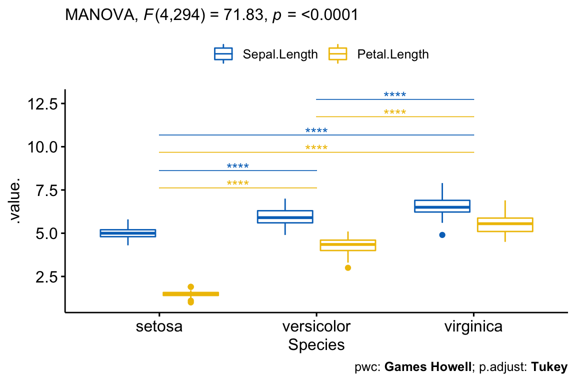
All pairwise comparisons between groups were significant for each of the outcome variable (Sepal.Length and Petal.Length).

# Visualization: box plots with p-values
pwc <- pwc %>% add_xy_position(x = "Species")
test.label <- create_test_label(
  description = "MANOVA", statistic.text = quote(italic("F")),
  statistic = 71.83, p= "<0.0001", parameter = "4,294",
  type = "expression", detailed = TRUE
  )
ggboxplot(
  iris2, x = "Species", y = c("Sepal.Length", "Petal.Length"), 
  merge = TRUE, palette = "jco"
  ) + 
  stat_pvalue_manual(
    pwc, hide.ns = TRUE, tip.length = 0, 
    step.increase = 0.1, step.group.by = "variables",
    color = "variables"
    ) +
  labs(
    subtitle = test.label,
    caption = get_pwc_label(pwc, type = "expression")
  )

Summary

This article describes how to compute and interpret one-way MANOVA in R. We show how to check the test assumptions and to perform post-hoc analyses.

References

Tabachnick, Barbara, and Linda.S. Fidell. 2012. Using Multivarite Statistics. 6th ed. Pearson.

Recommended for you

This section contains best data science and self-development resources to help you on your path.

Coursera - Online Courses and Specialization

Amazon FBA

Amazing Selling Machine

Free Training - How to Build a 7-Figure Amazon FBA Business You Can Run 100% From Home and Build Your Dream Life! by ASM

Books - Data Science

Our Books

Practical Guide to Cluster Analysis in R by A. Kassambara (Datanovia)
Practical Guide To Principal Component Methods in R by A. Kassambara (Datanovia)
Machine Learning Essentials: Practical Guide in R by A. Kassambara (Datanovia)
R Graphics Essentials for Great Data Visualization by A. Kassambara (Datanovia)
GGPlot2 Essentials for Great Data Visualization in R by A. Kassambara (Datanovia)
Network Analysis and Visualization in R by A. Kassambara (Datanovia)
Practical Statistics in R for Comparing Groups: Numerical Variables by A. Kassambara (Datanovia)
Inter-Rater Reliability Essentials: Practical Guide in R by A. Kassambara (Datanovia)

Others

R for Data Science: Import, Tidy, Transform, Visualize, and Model Data by Hadley Wickham & Garrett Grolemund
Hands-On Machine Learning with Scikit-Learn, Keras, and TensorFlow: Concepts, Tools, and Techniques to Build Intelligent Systems by Aurelien Géron
Practical Statistics for Data Scientists: 50 Essential Concepts by Peter Bruce & Andrew Bruce
Hands-On Programming with R: Write Your Own Functions And Simulations by Garrett Grolemund & Hadley Wickham
An Introduction to Statistical Learning: with Applications in R by Gareth James et al.
Deep Learning with R by François Chollet & J.J. Allaire
Deep Learning with Python by François Chollet

Version: Français

Back to Comparing Multiple Means in R

Comment ( 1 )

Evan

14 Mar 2023

This post was perfect! Thank you so much for navigating me through MANOVA!

Reply

Comparing Multiple Means in R